Probable Pattern

Two-Way Sorting

One of the popular ways to motivate a two dimensional model is to double sort your data based on quantiles. This makes empirical asset pricing models exceedingly easy to understand. If I had already defined the breakpoints of the sort, I could just use a function like “plyr” to apply a function like “mean” to the data subsets. For my application, I want to create five portfolios based on one characteristic and then form five portfolio within each of the first five based on another characteristic. To generalize from a 5×5 sort, I include the parameter q to allow for quarters or deciles. The x and y parameters are the column names of the characteristics you want to sort by. As you can see from the last line, I am sorting by CDS premium and liquidity premium. I use latex for my publication needs so I output the dataframe to xtable. I also use the awesome foreach package to speed things up a tiny bit but if you don’t use a parallel backend with foreach, then just replace “%dopar%” with “%do%”. Happy sorting!

require(foreach); require(xtable)
doublesort=function(data,x,y,q) {
 breaks1=quantile(data[,x],probs=seq(0,1,1/q))
 tiles=foreach(i=1:q,.combine=cbind) %dopar% {
 Q=data[data[,x]>=breaks1[i] & data[,x]<breaks1[i+1],y]
 breaks2=quantile(Q,probs=seq(0,1,1/q))
 foreach(j=1:q,.combine=rbind) %dopar%
  mean(Q[Q>=breaks2[j] & Q<breaks2[j+1]])
 }
 colnames(tiles)=foreach(i=1:q) %do% paste(x,i)
 row.names(tiles)=foreach(i=1:q) %do% paste(y,i)
 tiles
}
xtable(doublesort(data,"CDS","lp",5),digits=4)

Dashboards

Precious Metals Dashboard
This R script produces charts of Gold, Platinum, Palladium, and Silver.

# Charts Gold prices in USD from Oanda
require(Quantmod)
#fetch data
getSymbols(c("XAU/USD","XPT/USD","XPD/USD","XAG/USD"),src="oanda")
#setup the plot area, each TA is another graph
layout(matrix(1:4, nrow=2))
#charts to be included
chartSeries(XAUUSD,name="Gold (.oz) in USD", layout=NULL)
chartSeries(XPTUSD,name="Platinum (.oz) in USD", layout=NULL)
chartSeries(XPDUSD,name="Palladium (.oz) in USD", layout=NULL)
chartSeries(XAGUSD,name="Silver (.oz) in USD", layout=NULL)

Interest Rate Dashboard
Another R script that charts the last 36 months of the following interest rates: 1 year U.S. Treasury, 10 year TIPS, 30 year fixed mortgage, Prime, Moody’s Aaa Corporate, and Moody’s Baa Corporate.

library(quantmod)
getSymbols("DGS1",src="FRED") #1 Year US Treasury Daily Constant Maturity rate
getSymbols("DPRIME",src="FRED") #Daily Prime Loan Rate
getSymbols("DAAA",src="FRED") #Daily Moody's Aaa Corporate Bond Yield
getSymbols("DBAA",src="FRED") #Daily Moody's Baa Corporate Bond Yield
getSymbols("MORTG",src="FRED") #30 Year Conventional Mortgage Rate
getSymbols("FII10",src="FRED") #10 Year TIPS Constant Maturity
# Chart Data
layout(matrix(1:6, nrow=3))
chartSeries(last(DGS1,'36 months'),name="US Treasury 1 Year Constant Maturity",layout=NULL)
chartSeries(last(FII10,'36 months'),name="10 Year TIPS Constant Maturity",layout=NULL)
chartSeries(last(MORTG,'36 months'),name="30 Year Fixed Mortgage Rate",layout=NULL)
chartSeries(last(DPRIME,'36 months'),name="Prime Loan Rate",layout=NULL)
chartSeries(last(DAAA,'36 months'),name="Moody's Aaa Corporate Yield",layout=NULL)
chartSeries(last(DBAA,'36 months'),name="Moody's Baa Corporate Yield",layout=NULL)

Rolling Correlations
Chart rolling correlations with a 3 month window.

library(quantmod)
getSymbols(c("SPY","^DJI"),src="yahoo")
data=data.frame(SPY[,6],DJI[,6])
data=as.xts(data,order.by=as.Date(row.names(data),"%Y-%m-%d"))
c1=rollapply(data,65,cor,by.column=F)
Correlation=c1[,2]; chartSeries(Correlation)

First Database in R

The number of simulations I am now running in R consumes all the memory on my workstation causing it to freeze. While I would like to execute the simulations in smaller batches, I need to keep a record of the intermediate data generated which is currently being stored in arrays. One possible solution would be to generate many CSV files to store the intermediate data and read from those but reassembling the data for audit purposes would not be practical. After some excellent suggestions on Stack Overflow, I narrowed my options down to SQLite and MySQL databases with a preference for SQLite due to simplicity. Not being a command line purist, I thought the next step was to find a GUI for setting up the database. While SQLite Database Browser seemed to be the only FOSS GUI available, it requires the Qt library to run and I prefer not to install additional components on my Mac when possible. MySQL does have a FOSS GUI called MySQL Workbench and Thomas Henlich created a plugin for exporting to SQLite but it turns out that SQLite is easy enough to use without a GUI even if you have no prior database experience. The easiest way to get a handle on it is to use a known data set and learn how to send and retrieve it from SQLite using R code. I highly recommend trying to run the database from disk rather than memory since it provides a closer approximation to the problem you are likely to be solving.

Here’s a short example of reading a data set that is currently stored in a csv format, creating a SQLite database, writing the data into a table, and retrieving the information. Make sure that the RSQLite package is installed and active.

# Read data
dataset=read.csv("/yourdirectory/yourfile.csv",skip=1,header=TRUE)
# Create DB
testdb=dbConnect(SQLite(), dbname = "/yourdirectory/testdb.dat")
# Write the data set into a table called table1
dbWriteTable(testdb,"table1",dataset)
# List the tables available in the database
dbListTables(testdb)
# Remove the original data to free up memory
rm(dataset)
# Retrieve the entire table
dbReadTable(testdb,"table1")
# Retrieve the single column called series from the table
buf<-dbSendQuery(testdb,"select series from table1")
testing<-fetch(buf,n=-1); dbClearResult(buf)
dbDisconnect(testdb); rm(buf,testdb)

SQL queries generate a result that is stored in a buffer. Fetch gets data from the buffer and directs it to the variable within R. Before doing another SQL query on the same data, you need to clear the buffer using dbClearResult. This process gets to be a pain when making many queries but the SQLiteDF package has an excellent method for treating SQLite database tables as data frames. I also recommend reading about the TSSQLite package if you are using time series data and work with zoo objects.

Introduction to Bootstrapping with R

Bootstrapping is a process where your original data is re-sampled to produce a distribution of a single statistic such as the mean. The Wikipedia article has more information here. Since time-series data often have some amount of dependency from one period to the next, we re-sample the original data in blocks. Assuming your data set has 100 observations and the block size is 6, we start at a random observation and sample the next 6 observations. We start at another random observation and sample another consecutive 6 observations repeating this process until we have 100 observations which is called a replicate. (When n/block size is not an integer, we get a shorter block at the end.) The statistic (in this case the mean) is calculated for each replicate. Multiple replicates are used to construct a distribution of the statistic so we can now draw inferences from the data. Since the function tsboot only returns the result of bootstrapping the statistic, you will need to find the actual data in each replicate in order for others to reproduce your results. The original data is not stored in the output but the index of the original data can be obtained using the boot.array command. Before you use your newly generated data, you will want to check whether the settings you used such as the number of replicates and the block size are adequate to capture the statistic of interest. A simple plot of the tsboot output will do the trick. For a more in-depth analysis of the proper block size, check out the b.star function in the np package and research by Poltis and White (2004). When you tire of calculating basic statistics, tsboot will accept a custom function that can be used instead of a command such as “mean” to calculate the statistic. The December 2002 edition of R News has a good overview of the boot package.

require(boot)
# Simple example of bootstrapping mean from 100 random numbers
x <- rnorm(100)
y <- tsboot(x, mean, R=10, l=20, sim=”fixed”)
# histogram of R number of statistic (index = t of interest from tsboot output)
plot(y, index=1)
# matrix of the data index (column) occurring in bootstrap replicate (row)
y.array <- boot.array(y)
# Write to CSV
write.csv(y.array,”/yourdirectory/yourfile1.csv”)
write.csv(x,”/yourdirectory/yourfile2.csv”)

Timing csv File Reading in R and Python

I am currently working with trade data organized in large csv files. I took this as an opportunity to learn the Pandas package in Python mostly for the HDF5 integration. As a sanity check, I decided to time three methods: read.csv in R base, fread in the data.table package in R, and read.csv in the Pandas package in Python. Let me first say that I am not a programmer. This test is not a definitive benchmark of the three methods. It is a benchmark of the “out-of-the-box” functionality available to the non-programmer trying to use code to get shit done. I used time.time() in Python and proc.time() in R to read 10,000,000 rows of mixed data types. Without further ado, here are the results: read.csv in R took 131.45 seconds, read.csv in Pandas took 27.741 seconds, and the winner was fread in the data.table package clocking in at 14.018 seconds. Unfortunately, fread needs more TLC in determining data types and missing values. Pandas just works right the first time. I also prefer the time manipulation in Pandas compared to the XTS package in R but not enough to deal with two languages in one project.

Quebec City

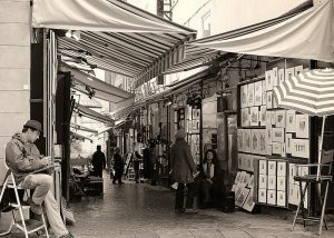
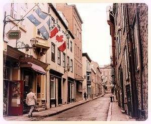
QC_walking Quebec City is the only walled city in North America. I could have spent a week just bouncing from cafe to cafe eating crepes but I was there for an academic conference. Parliament and the citadel are worth a visit. Both the fortifications and the Terrasse Dufferin are lovely walks in good weather. The city is built on a hill so bring some good walking shoes and don’t miss the farmers market. If you have time, take a bicycle ride along the river path.

QC_street

Mira

A good samba is light and floats through the air without losing its rhythmic grounding. While the video is fine, I have to admit that I loved this song before the video and I don’t think it added much to the song.

A Capriote

I visited the Museum of Fine Arts in Boston the other day. For non-art fans, John Singer Sargent was a great American portrait painter. This is one of my favorite paintings although I am sure his other work is more appreciated.

Managerial Game Theory

One of the first models covered in game theory is the Prisoner’s Dilemma. I’m sure you’ve heard of it or at least recognize it from episodes of Law and Order. Let’s look at the simple model with 2 individual players so we can eliminate mixed strategy equilibria and focus strictly on pure strategies.

The two strategies for each player are “productive” and “exploitive”. The payoffs for the two players can be summarized on the usual grid.

		Employee
		Productive	Exploitive
Manager	Productive	1,1	0,2
Manager	Exploitive	2,0	0,0

One possible economic interpretation of this payoff structure is the ratio of compensation to work output. A ‘1’ represents compensation that accurately prices the employee’s output. A ‘2’ or a ‘0’ represent either excessive compensation for the same output or excessive output for the same compensation. Consistent with these payoffs, the manager prefers to get as much output as possible for as little compensation as possible while the employee prefers the opposite.

In a single period game, the dominant strategy of both players is to choose the exploitive relationship but if both players believe that they will repeat the game, the productive strategy produces the maximum utility for both players. It is fairly safe to assume that both players will begin with the productive strategy since they believe that the game will be played multiple times. The utility of one player starting off with an exploitive relationship and playing until time ‘t’ would be

U= Σ[2, 0/(1+r), 0/(1+r)², 0/(1+r)³,…0/(1+r)^t]

where r is the discount rate under which the player values the next period payoff in the current period. As we can see, the utility of this player is 2 so this player will only begin with an exploitive relationship if he/she believes that

2 > Σ[1, 1/(1+r), 1/(1+r)², 1/(1+r)³, 0/(1+r)^k…0/(1+r)^t]

where k+1 is the number of times the game is played before the other player switches to an exploitive strategy. Without an extremely high discount rate ‘r’ the player needs to trust that the other will not switch strategies for relatively few game iterations. So few iterations are needed that I would say that any player with a rational discount rate would start with a productive relationship. Unfortunately, it does not follow that both players will continue to pursue a productive relationship beyond the first few iterations of the game.

The player with the higher discount rate will switch strategies first in order to realize a higher present value of the increased payoff of ‘2’. At this point, both players will pursue the exploitive relationship until the end of the game. Since the discount rate may be interpreted as a measure of risk aversion, the player with greater risk aversion will be the first to pursue an exploitive relationship.

While there are many real world complications with the enforcement of the payoff structure and possible reputational effects for future working relationships, it is important to understand the ease with which reputational effects may be mitigated through HR disclosure policies. Excessive faith in employee controls and risk management policies can lead to risk averse managers and employees both pursuing exploitive relationships. Employees and managers may want to engage in working relationships with riskier counterparties if they want to remain productive.

The Decreasing Marginal Utility of Donuts

This morning I ran through the Dunkin Donuts to pick up two donuts for me and two donuts for my wife. Four donuts cost $3.85 while 6 donuts cost a little over $4.00. The cashier tried to convince me that buying 6 donuts would be cheaper. Understandably, the cashier would not know that I was ordering for only two people or that we prefer not to stuff ourselves with more than two donuts each. Still, I feel like the cashier never quite believes that I understand the cost per donut is lower with an order of 6 versus 4 but that it is entirely rational to base decisions on total cost rather than unit cost.